Mobile/Whole-Body Manipulation with KUKA youBot
MATLAB, Manipulation, Motion Planning, Controls, CoppeliaSim, KUKA youBot
Overview
This was the Capstone Project for the course: ME 449 Robotic Manipulation by Dr. Kevin Lynch at Northwestern University.
In this project, I wrote software that plans a trajectory for the end-effector of a KUKA youBot mobile manipulator (a mobile base with four mecanum wheels and a 5R robot arm), performs odometry as the chassis moves, and performs feedback control to drive the youBot to pick up a block at a specified location, carry it to a desired location, and put it down.
Functions from the modern-robotics library were used in this project.
The final output of my software is a comma-separated value (csv) text file generated using a MATLAB script that specifies the configurations of the chassis and the arm, the angles of the four wheels, and the state of the gripper (open or closed) as a function of time. This specification of the position-controlled youBot was then tested on the CoppeliaSim simulator. Here, the ODE physics engine was used to simulate contact dynamics and inertial forces.
The program takes as input:
- The initial resting configuration of the cube object (which has a known geometry), represented by a frame attached to the center of the object
- The desired final resting configuration of the cube object
- The actual initial configuration of the youBot.
- The initial configuration \(T_{se}\) of the reference trajectory for the end-effector frame of the youBot
The program’s output is:
- A csv file which, when “played” through the CoppeliaSim scene, drives the youBot to successfully pick up the block and put it down at the desired location.
- A data file containing the 6-vector end-effector error as a function of time
Personal Motivation
In my junior year at BITS Pilani, I began reading Dr. Kevin Lynch’s book on Modern Robotics. In the weeks that followed, I just could not put the book down and I solved every single exercise in the foundational chapters. The book’s formal, systematic, and comprehensive approach to robotics was what I resonated with the most and is precisely the mindset I wanted to adopt as a roboticist. Since then, I have referred to it throughout my experiences in controlling and designing robots, and is why I decided to pursue an MS in Robotics at Northwestern. In my first quarter here, I actually got to attend Dr. Lynch’s Robotic Manipulation Class, and undertake this final project.
Kinematics of the KUKA youBot
The configuration of the frame {b} of the mobile base, relative to the frame {s} on the floor, is described by the 3-vector \(q = (\phi, x, y)\) or the \(SE(3)\) matrix:
\[T_{sb}(q) = \begin{bmatrix} cos \phi & -sin \phi & 0 & x \\ sin \phi & cos \phi & 0 & y \\ 0 & 0 & 1 & 0.0963 \\ 0 & 0 & 0 & 1 \end{bmatrix} <br> <figure align = "center"> <img src="https://hades.mech.northwestern.edu/images/thumb/3/33/Yb-book.png/1200px-Yb-book.png" width="65%"/> <figcaption><em>Fig. 1. This figure illustrates the arm at its home configuration (all joint angles zero) and the frames {s}, {b}, {0}, and {e}. For the image on the right, joint axes 1 and 5 (not shown) point upward and joint axes 2, 3, and 4 are out of the screen. <a href="https://hades.mech.northwestern.edu/index.php/File:Yb-book.png" target="_blank">[Image Source]</a></em></figcaption> </figure> <br>\]The wheel numbering and forward driving and “free sliding” direction \(\gamma\) of each wheel is indicated as:

Dynamics Simulation in CoppeliaSim
The CoppeliaSim scene used for the capstone project is the first scene in which we’ve used CoppeliaSim’s ability to simulate bodies in contact. A “physics engine” simulates the motions of bodies when forces are applied to them, and when they make contact or collide with each other. Physics engines also handle articulated bodies with joints and other constraints. Here, ODE has been used as the physics engine.
Rigid Bodies
In CoppeliaSim, each rigid body is classified as either respondable or non-respondable:
- respondable: The body can make contact and collide with other bodies.
- non-respondable: The body can pass through other bodies. Thus if a respondable body and a non-respondable body overlap, or if two non-respondable bodies overlap, there is no collision. If two respondable bodies make contact, however, forces will try to keep them from penetrating each other.
In this scene, only the floor, the gripper fingers, and the cube are respondable. All other bodies are non-respondable.
In addition, each rigid body can be classified as dynamic or non-dynamic:
- dynamic: The body has mass and inertial properties that are used to compute its motion. For example, as shown in the image to the right, you can click on “Cuboid_initial” to learn about the mass properties of the cube in Scene 6. You can also learn about material properties, like “friction values.” (The simulated friction coefficient of two bodies in contact is calculated as the product of the friction values of the two materials. This is a simple, but non-physical, way to come up with a friction coefficient for two bodies in contact without having to specify a friction coefficient for every possible pair of materials in contact.)
- non-dynamic: The body’s motion is not computed according to dynamics computed by the physics engine.
In this scene, only the gripper fingers and the cube are dynamic.
Joints
In this scene, each joint is either in torque/force mode or passive mode:
- torque/force mode: In torque/force mode, the motion of the joint is controlled by a torque or force applied by an actuator, possibly governed by a PID control law, for example.
- passive mode: In this mode, the joint is kinematically controlled to go to specified positions, without reference to forces or torques.
In this scene, all joints are in passive mode, except for the two joints controlling the gripper motion. The PID control dynamics for these passive joints has been simulated directly in the trajectory generator.
Trajectory Generation
The code pieces together a reference trajectory using various keyframes as a Quintic Via Point Trajectory. Let the trajectory be specified by \(k\) via points, with the start point occurring at \(T_1 = 0\) and the final point at \(T_k = T\). At each via point \(i ∈ {1, . . . , k}\), the user specifies the desired position \(β(T_i) = β_i\) and velocity \(\dot{\beta}(T_i) = \dot{β}_i\). The trajectory has \(k −1\) segments, and the duration of segment \(j ∈ {1, . . . , k − 1}\) is \(∆T_j = T_j+1 − T_j\). The joint trajectory during segment j is expressed as the \(5^{th}\)-order polynomial:
\(\beta(T_j + ∆t) = a_{j0} + a_{j1}∆t + a_{j2}∆t^2 + a_{j3}∆t^3\).
Here,
\[\begin{align*} a_{j0} &= β_j,\\ a_{j1} &= \dot{β}_j, \\ a_{j2} &= \frac{3\beta_{j+1} - 3\beta_{j} - 2\dot{\beta_j}∆T_j - 2\dot{\beta}_{j+1}∆T_j}{∆T_j^2}, \\ a_{j3} &= \frac{2\beta_{j} + (\dot{\beta}_{j} + 2\dot{\beta}_{j+1})∆T_j - 2\beta_{j+1}}{∆T_j^3}. \end{align*}\]The 8 segments of the trajectory comprise:
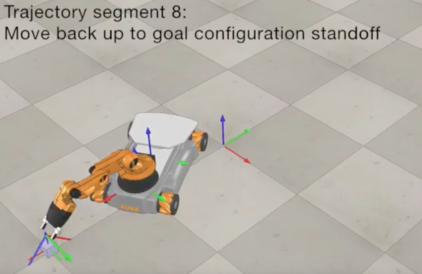
- Moving the gripper from its initial configuration to a “standoff” configuration above the block.
- Moving the gripper down to the grasp position.
- Closing the gripper.
- Moving the gripper back up to the “standoff” configuration.
- Moving the gripper to a “standoff” configuration above the final configuration.
- Moving the gripper to the final configuration of the object.
- Opening the gripper.
- Moving the gripper back to the “standoff” configuration.
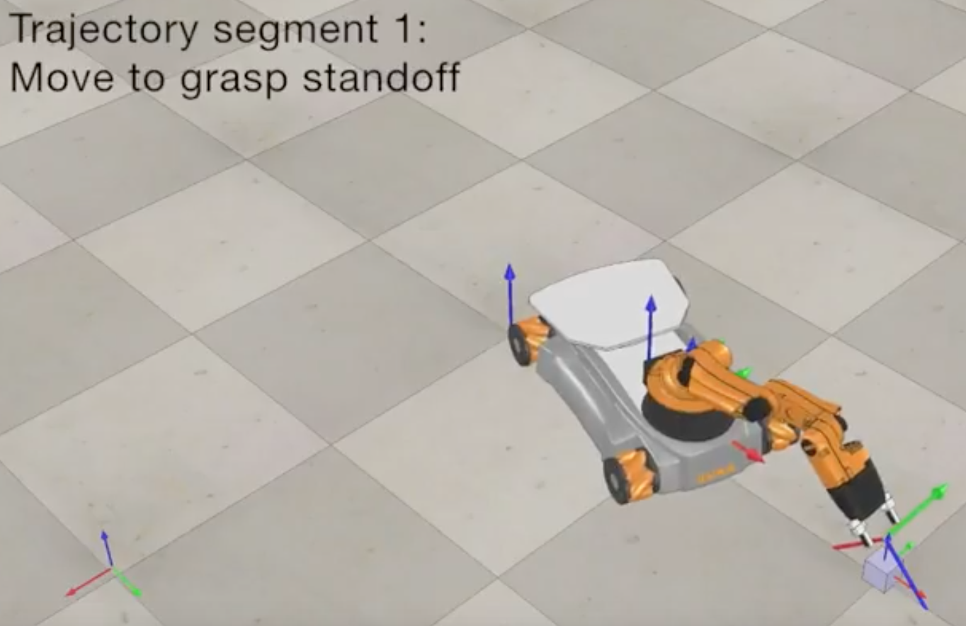

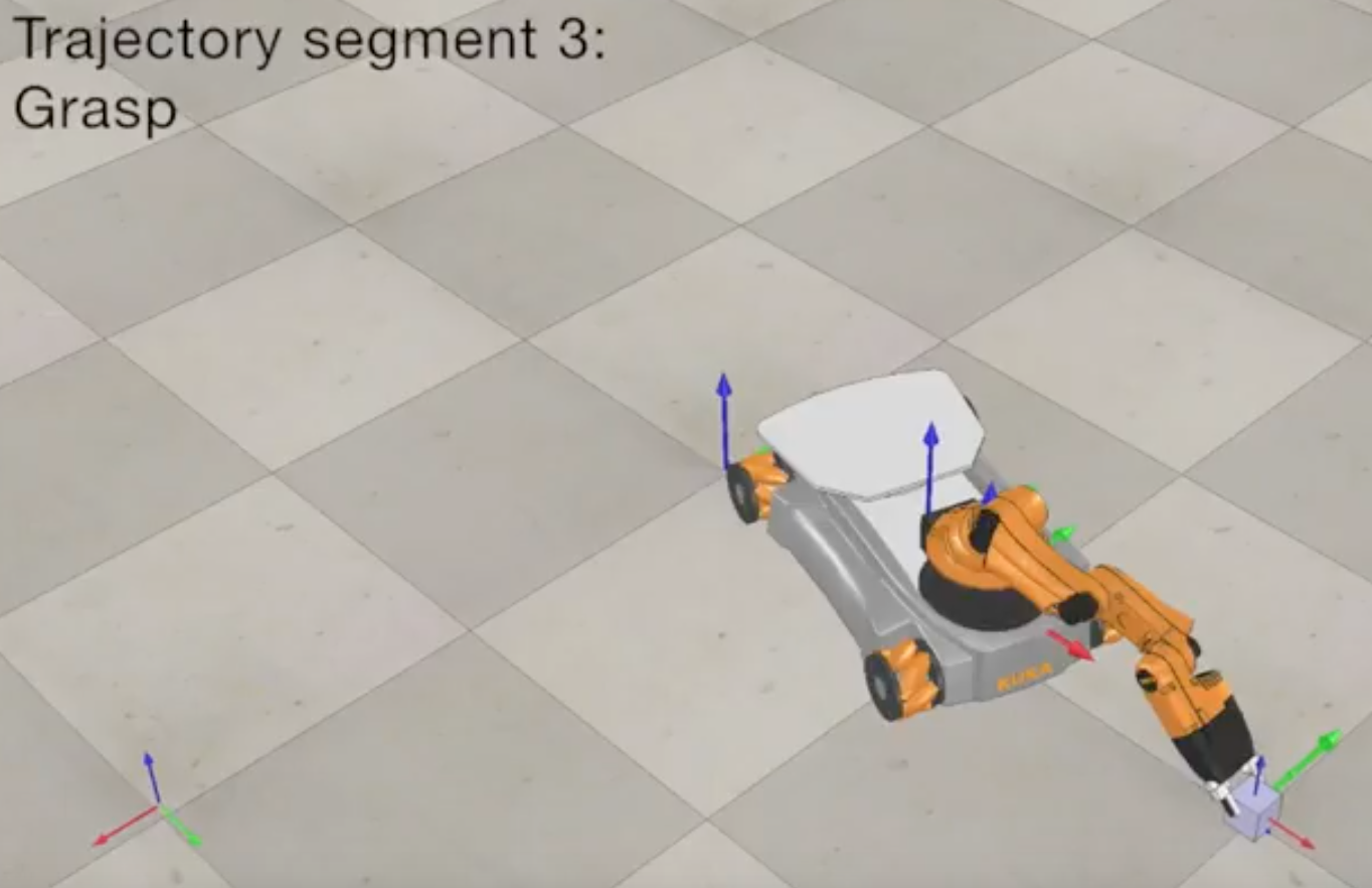

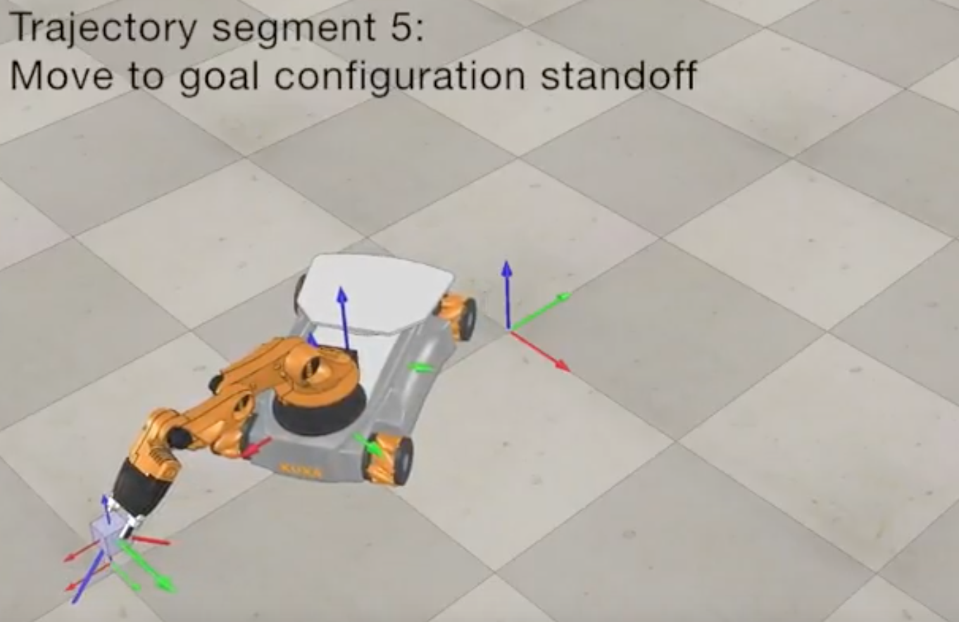
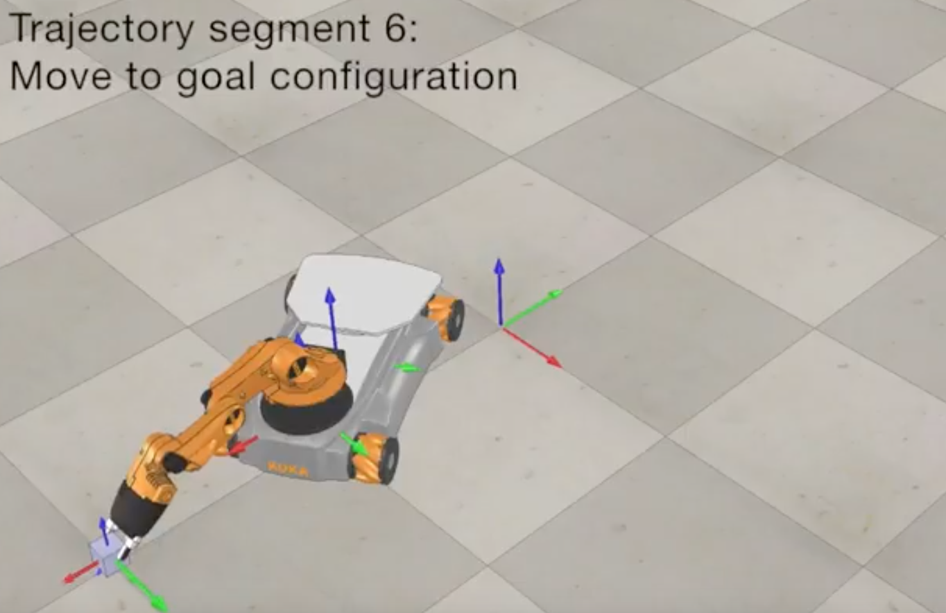

Feedback Control
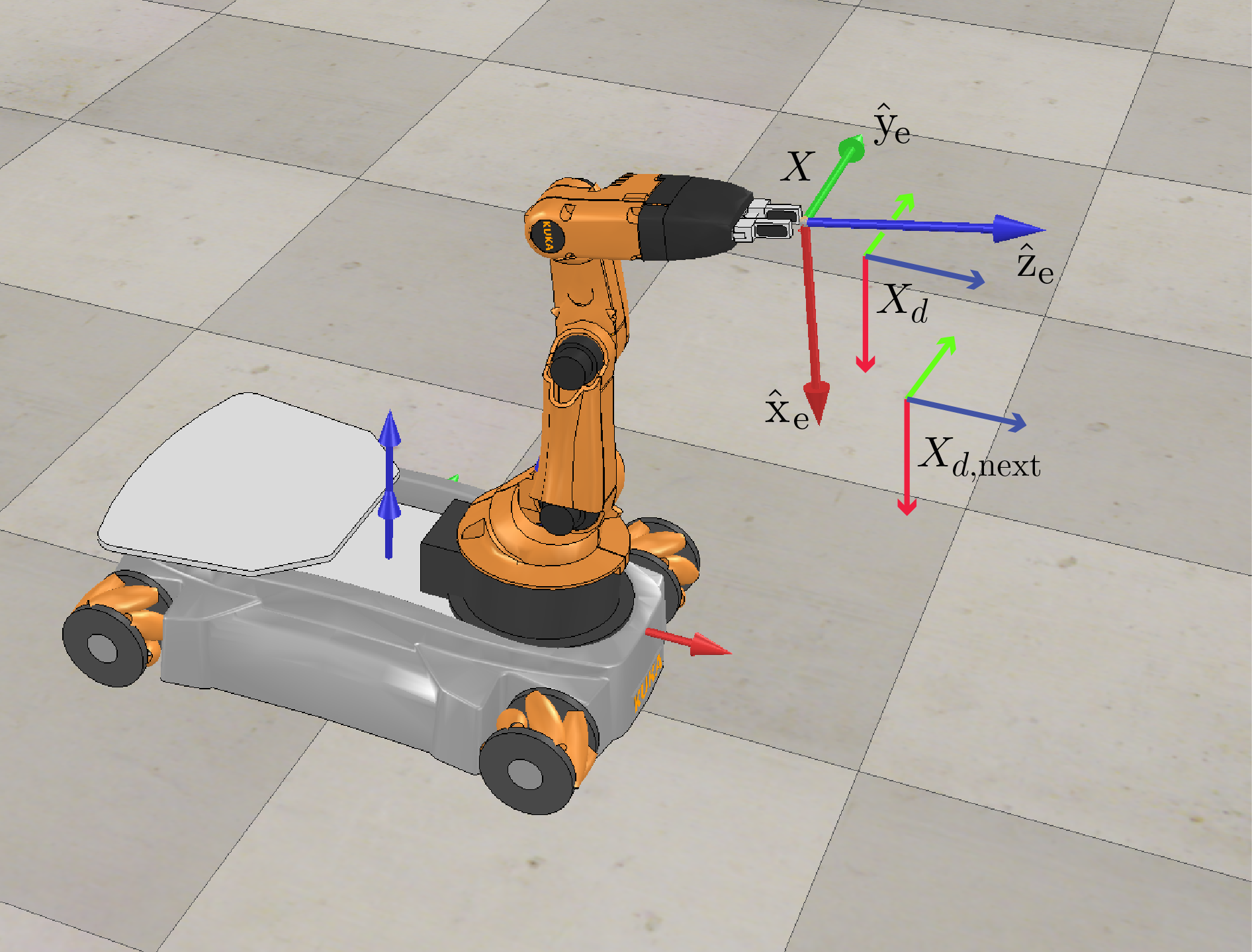
The feedback control law for the system:
\[\mathcal{V}(t) = [Ad_{X^{-1}X_{d}}]\mathcal{V}_{d}(t) + K_{p}X_{err}(t) + K_i\int_{0}^{t}X_{err}(t)dt\]takes in:
- \(X\): the actual end effector configuration.
- \(X_d\): the desired end effector configuration. And hence, \(X_{err} = log(X^{-1} X_d)\)
- \(X_{d,next}\): the desired configuration at the next time step. And hence, \([V_d] = (1/∆t)~log(X^{-1}_d X_{d,next})\)
to give us the commanded end-effector twist \(\mathcal{V}\) at every time step.
To turn this into commanded wheel and arm joint speeds \((u, \dot{\theta})\), we use the pseudoinverse of the mobile manipulator Jacobian \(J_e(\theta)\):
\[\begin{bmatrix} u \\ \dot{\theta} \end{bmatrix} = J^{\dagger}_e(\theta) \dot{\theta}\]Reference